3. Finite Markov Decision Processes

3.1 The Agent–Environment Interface

 

The function p defines the dynamics of the MDP.

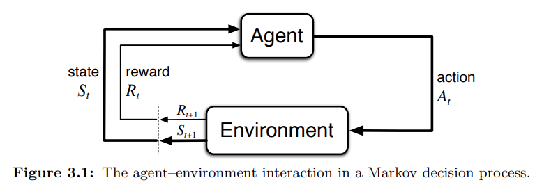
for all $s' , s \in S, r \in R$, and $a \in A(s)$. The function p defines the dynamics of the MDP. Whereas bandit problem doesn't change the state of the environment, in reinforcement learning the action of the agent changes the state of the environment.

• State Trainsition Probability: (use this when reward is deterministic)

• The expected rewards for state–action pairs:

• the expected rewards for state–action–next-state triples:

3.2 Goals and Rewards

That all of what we mean by goals and purposes can be well thought of as the maximization of the expected value of the cumulative sum of a received scalar signal (called reward). 

3.3 Returns and Episodes

Returns

In the simplest definition return is the sum of future rewards. $T$ is the final time step.

Episodes

When the agent–environment interaction breaks naturally into subsequences, we call it episodes. Each episode ends in a special state called the terminal state, followed by a reset to a standard starting state or to a sample from a standard distribution of starting states.

• episodic task: $T \neq \infty$
• continuous tasks: $T = \infty$ 

cf) in continuous tasks we need to use discounted return because return could easily go to infinity.

where $\gamma$ is called a discounted rate. ($ 0 \leq \gamma \leq 1$)

discouted return in recurrence relation

3.4 Unified Notation for Episodic and Continuing Tasks

diagram for unified notation

Unified notation for return

3.5 Policies and Value Functions

• Policies

Formally, a policy is a mapping from states to probabilities of selecting each possible action. If the agent is following policy $\pi$ at time $t$, then $\pi(a|s)$ is the probability that $A_t = a$ if $S_t = s$. Like $p_\pi$ is an ordinary function; the “|” in the middle of $\pi(a|s)$ merely reminds that it defines a probability distribution over $a \in A(s)$ for each $s \in S$. Reinforcement learning methods specify how the agent’s policy is changed as a result of its experience.

 

• State-value function

state-value function

• Action-value function

action-value function

Bellman equation for state-value function

exercise) The value of a state depends on the values of the actions possible in that state and on how likely each action is to be taken under the current policy. We can think of this in terms of a small backup diagram rooted at the state and considering each possible action:

3.6 Optimal Policies and Optimal Value Functions

optimal state-value function

optimal action-value function

optimal policy

bellman optimality equation for $\pi_*$

bellman optimality equation for $q_*$

:Backup diagrams for $\nu_*$ and $q_*$